Risk Premiums and Risk Aversion

Risk level of an investor is determined by degree to which investors are willing to commit funds
Risk aversion is how reluctant you are in investing.
If T-Bill denotes the risk-free rate, rf, and variance denotes volatility of returns then:
The risk premium of a portfolio is: E(rp) - rf
In other words, expected return of portfolio minus risk-free rate.

To quantify the degree of risk aversion with parameter A:
 

The Sharpe (Reward-to-Volatility) Measure

This sharpe ratio is known to be used by mutual/hedge fund managers. This shows how much extra/additional return (excessive return or premium) you are earning when you bear a unit of risk in an investment. The Sharpe ratio has as its principal advantage that it is directly computable from any observed series of returns without need for additional information surrounding the source of profitability.

Risk and risk premium

Risk is uncertainty. When you make an investment, there is always a risk associated with it whether it is a bond, stock, fund, etc. Risk arises from uncertainty. We don't know market direction next year. As a matter of fact, we don't even know how market will drop/raise our stock price tomorrow. Risk can be separated into 2 different types. One is an internal risk. This is also known as a business specific risk, where uncertainty comes from the company and its operation. The other one is a market risk. This is an external risk that you will have to bear.

Scenario Analysis and  Probability Distributions
In order to examine risk, we can look at the risk/uncertainty using probability. Here 3 important variables that you need to know before moving on the analysis.
1) Mean: most likely value
2) Variance or standard deviation
3) Skewness

This picture demonstrates famous concept known as "normal distribution." The normal distribution is an absolutely continuous probability distribution whose cumulants of all orders above two are zero. Note that norm. distribution has mean equals to median.
In probability theory and statistics, skewness is a measure of the asymmetry of the probability distribution of a real-valued random variable. skewness value can be positive or negative, or even undefined. Qualitatively, a negative skew indicates that the tail on the left side of probability density function is longer  than the right side and the bulk of the values (including the median) lie to the right of the mean. A positive skew indicates that the tail on the right side is longer than the left side and the bulk of the values lie to the left of the mean.

Measuring Mean: Scenario or Subjective Returns

p(s) = probability of a state
r(s) = return if a state occurs
1 to s states
This is a formula to calculate expected return (subjective/scenario return), which is equals to multiplication of each state's probability (in decimal) and return. After you get each value, sum them up to get final E(r) value.

Numerical Example: Subjective or Scenario Distributions

State    Prob. of State    rin State
    1            .1        -.05
    2            .2        .05
    3            .4        .15
    4            .2        .25
    5            .1        .35

    E(r) = (.1)(-.05) + (.2)(.05)...+ (.1)(.35)
    E(r) = .15 or 15%


Measuring Variance or Dispersion of Returns
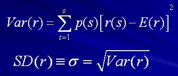
Variance is used as one of several descriptors of a distribution. It describes how far values lie from the mean.

Var = sum of probability (in decimal) multiplied by outcome of individual return minus average. And Standard deviation is simply a square root of variance.

Using the same example above,

Var =[(.1)(-.05-.15)2+(.2)(.05- .15)2...+ .1(.35-.15)2]
Var= .01199
S.D.= [ .01199] 1/2 = .1095 or 10.95%

Quoting Conventions

APR =  annual percentage rate
    (periods in year) X (rate for period)
EAR = effective annual rate
    ( 1+ rate for period)^Periods per yr - 1
Example: monthly return of 1%
    APR = 1% X 12 = 12%
    EAR = (1.01)^12 - 1 = 12.68%

Dollar weighted returns

Here are some characteristics of dollar weighted returns.
-It considers changes in investment
-Initial Investment is an outflow (money going out from your pocket)
-Ending value is considered as an inflow (money coming into your pocket)
-Additional investment is a negative flow (Again, money leaving your pocket)
-Reduced investment is a positive flow (Again, money coming back to your pocket)




Dollar weighted return is nothing more than a IRR.
Internal Rate of Return (IRR) is the discount rate that results in present value of the future cash flows being equal to the investment amount.

Example

When you compute the IRR, this is the rate of return at which the net present value of project/investment is zero. In other words, if the internal rate of return exceeds the cost of financing the project, then the investment is profitable.

We can also approach it from NPV perspective.
 
NPV = Sum of CFt/ (1+ Rt)^t from period t=0 to n.
Whereas NPV = Net present value and CFt = Cash flow at time t.

When the rate of return is smaller than the IRR rate Rt then the investment is profitable (meaning NPV > 0 ). Otherwise, investment is not profitable.

IRR can also be a good measurement when considering multiple investment with a limited budget.
So if you have two different stocks in mind but only have a few hundred bucks then you would compute IRR and see which one has higher IRR.
However, there are some limitations with dollar weighted returns.
If cash flow changes from positive to negative or from negative to positive, IRR for investment cannot be calculated. Additionally, when you use IRR to evaluate multiple investment, result might indicate different ranking than NPV.
For instance NPVa = 50 and NPVb = 100 but IRRa = 5 % and IRRb = 3.6 %
In this case, NPV indicate that investment b is more profitable but IRR says a is better.
Which one should you choose?
If NPV and IRR give different result then NPV always rules over IRR. So investment b is superior.
This is because of IRR's weaknesses. First IRR uses single discount rate failing to accommodate changes in the rate. Second, IRR sometimes cannot be computed with mixture of positive and negative cash flow. And lastly, discount rate is sometimes unknown. You compare IRR to discount rate and then proceed to make an investment if IRR> discount rate. But if discount rate is unknown or cannot be applied for whatever reason then IRR does not work. On the other hand, NPV is inherently complex and requires assumption at each stage. If NPV > 0 then we know investment is worthwhile. This is why NPV is superior than IRR.

Returns using arithmetic and geometric average

Arithmetic
rA = (r1 + r2 + r3 + ...rN) / N
rA = Arithmetic return
r1 = return 1, r2 = return 2, rN = return N, N = total number of returns
Example
rA = ( .10 + .25 - .20 + .25) / 4 = .10 or 10 %

Geometric
rg = {[(1+r1) (1+r2) .... (1+rn)]}^ 1/n - 1 
Example
rg = {[(1.1) (1.25) (.8) (1.25)]}^ 1/4 - 1
    =  (1.5150) 1/4 -1 = .0829 =  8.29%


Note that arithmetic average works better when each number is independent whereas geometric is a better choice if numbers are dependent to each other.
For instance, lets say you are trying to calculate average for annual stock returns over fiver year period. Each year's stock return is not independent of past year's performance. If you incur loss in one year then you have less capital to generate return following year. For this reason, geometric average may give more accurate performance of your portfolio.

Risk and returns

We all know that risk and return have a direct relationship. If you want a bigger return then you must be willing to take additional risks that come along with it.
Let us see how to compute rate of return.
Holding period return for stock
HPR = (P1-P0+D1) / P0 
Whereas P0=beginning price, P1= ending price, D1 = dividend
This return shows what % you earned during the stock holding period.
Example
Ending price = 24
Beginning price = 20
Dividend = 1
HPR = (24-20+1) / 20 = 25%
This is for a single period. In contrast when you want to measure return over multiple periods, you may need to measure how your investment performed over a preceding five-year period. Note that return measure is more ambiguous in this case.
Here's the example of multiple period return.

Leverage

In finance, leverage is any technique that is used to multiply gain or loss. Common usage of leverage is borrowing money to finance investment. For instance, let us say you bought 100 shares of stock A trading at $10. Total investment value is $1000. If the stock price increases from $10 to $15 then you have total investment value of $1500. So HPR would be (1500-1000)/1000 = .5 or 50 %. Now if you leverage your investment by borrowing money from your broker, return would be different. Let us say you borrow $1000 from Schwab and buy additional 100 shares at the same price $10 then you have total investment worth $2000. Again the stock price rises from $10 to $15. Here your total investment value becomes $3000. Subtract the borrowed fund $1000, which you will have to repay. Then you have final value of $2000. Your HPR would be (2000-1000)/1000 = 1 or 100 %. By borrowing half of your investment fund, you just doubled your return.

Case 1
100 shares at $10 = $1000 total
If stock price increases from $10 to $15
HPR = ($1500 - 1000)/ 1000 = .5 or 50 %

Case 2
100 shares at $10 = $1000
Additional 100 shares at $10 = $1000 ->borrowed fund from Schwab
Total investment value = $2000
If stock price increases from $10 to $15
HPR = ($3000 - 1000 - 1000) / 1000 = 1 or 100%

It is very important to acknowledge that leverage also works the same way in negative return. So that means if a half of your investment is leveraged then your profit or loss will be doubled. If stock price in the above declined from $10 to 5 then would have -50% return in the first case and -100% return in the second case.

Note that margin rate (interest you need to pay for borrowing fund) is not included in the calculation.

Leverage can be an excellent way to boost your return while it imposes a significant amount of risk. Shrewd investors must be careful using leverage and be willing to accept the risk that comes along.